Follow the numbers through an AI chip

When an AI model streams a reply, every new token has to be built from numbers moving through memory and compute. The surprising part is that the math is not always the slowest or most expensive piece. Often, the hard part is getting the right numbers to the right place quickly enough.

That is why AI chips are designed less like general-purpose computers and more like carefully arranged paths for data. To understand them, it helps to follow the numbers: from memory, into on-chip storage, through matrix engines, across pipeline stages, and finally into the next token you see on screen.

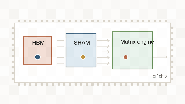
That physical map matters because the chip is fighting four related limits: arithmetic, data movement, synchronization, and memory bandwidth. The design keeps returning to the same question: what has to move next, and what can the chip change to make that movement cheaper?

The operation everything repeats

Most neural network layers eventually become matrix multiplication. Matrix multiplication looks complicated on paper, but the hardware keeps repeating one small operation: multiply two values, then add the product into a running sum. That is a multiply-accumulate, or MAC.

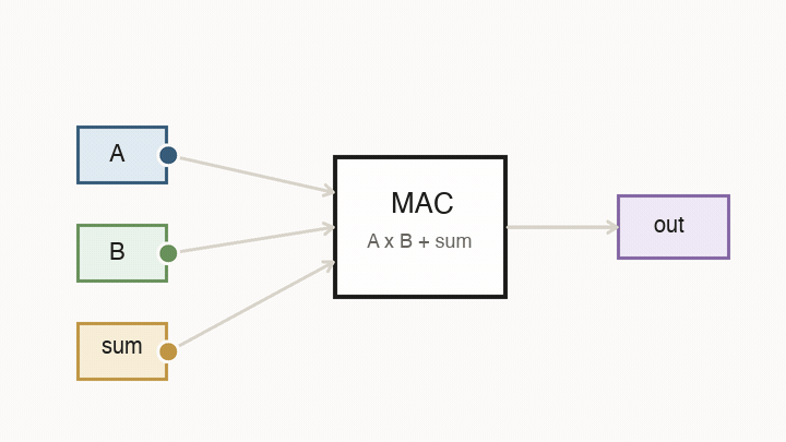
This is why AI chips dedicate so much area to matrix engines. They are not trying to execute arbitrary code as flexibly as a CPU. They are trying to do this one calculation at enormous scale, with data arriving in a predictable pattern.

If MACs were the whole story, the answer would be easy: put as many MAC units on the chip as possible. The rest of the article is about why that is not enough.

Why lower precision helps

The first way to fit more arithmetic onto a chip is to make each operation smaller. At the bit level, multiplication creates partial products. An 8-bit by 8-bit multiply has 64 bit-level products. A 4-bit by 4-bit multiply has 16.

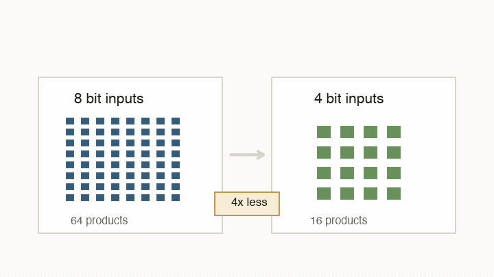
That is the hardware reason lower precision is valuable. If a model can tolerate 8-bit, 6-bit, or 4-bit values in the right places, each multiply can use less silicon and less energy. The accumulator often stays wider, because summing many products is where error can pile up.

Lower precision is not automatically better. It buys smaller math circuits and more throughput, but it leaves less numerical room. Modern AI systems spend a lot of effort finding where that trade is safe.

The next problem is more surprising: after you shrink the math, the wires and selectors around the math can become the bigger cost.

The hidden cost is movement

On a general-purpose processor, software needs flexibility. An instruction might read from many possible registers and write back to many possible places. The hardware that chooses those paths uses multiplexers, routing wires, and control logic.

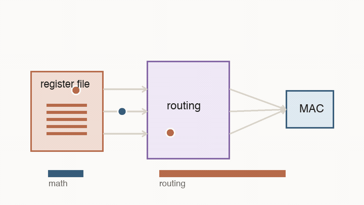
This is the first major shift from CPUs to AI accelerators. A CPU is designed to handle unpredictable instruction streams. An AI accelerator is designed around a known pattern: move blocks of numbers into the right place, multiply them, reuse them, and avoid unnecessary trips through large shared structures.

This is the point of following a number instead of just counting operations. A multiply that happens next door is cheap. The same multiply after a long trip through memory and routing logic is not.

Systolic arrays make reuse physical

A systolic array is a grid of small compute cells. Each cell holds a weight, receives an input, multiplies, adds to a partial sum, and passes values to neighboring cells.

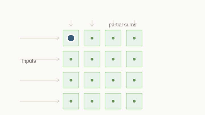
The important part is not the grid shape by itself. The important part is that reuse becomes physical. Instead of fetching every value from a central register file for every multiply, neighboring cells hand values to each other.

This changes what “fast” means. A value loaded into the array can contribute to many MACs before it travels far. The chip is no longer paying the full movement cost for every individual multiply. The hardware is shaped like the calculation.

Clocks, pipelines, and latency

The same idea applies to time. Digital chips do not let signals drift around forever. They use registers as checkpoints. On every clock tick, a register captures the value that has arrived at its input and holds it steady for the next stage.

That creates a deadline. Between two ticks, a value must leave one register, pass through wires and logic gates, and settle at the next register. If the path is too long, the chip cannot safely run the clock faster. The answer may arrive after the next tick, which means the next register captures the wrong thing.

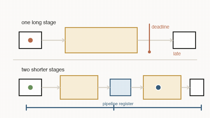
Pipelining is the standard fix: add another register in the middle. That does not make one value finish sooner. It splits the route into shorter stages, so each stage can meet a faster clock. After the pipeline fills, the chip can accept a new value every tick and produce a new result every tick.

The trade-off is latency. One value now takes more clock cycles to reach the end, even though the whole pipeline has higher throughput. This distinction matters: throughput is how many values the system can process once it is full; latency is how long one value waits from start to finish.

There is another catch. If a value feeds back into itself every cycle, as in an accumulator, you cannot always insert a register without changing the meaning of the computation. The chip designer is not just adding speed. They are deciding where time boundaries can be placed without breaking the math.

The same trade shows up when a model is spread across multiple chips or racks. Pipeline parallelism can help fit a larger model by putting different layers on different chips. But during decode, tokens are sequential: token 51 needs token 50 first. If a token has to cross several pipeline stages or network hops, those waits stack up in the user-visible latency.

Model serving is memory-shaped

Now the chip-level ideas turn into the behavior you feel in an AI product. When you ask a model a question, serving has two very different phases: prefill and decode.

Prefill processes the prompt you sent in. All of those input tokens are already known, so the system can push a large block of work through the matrix engines. During this pass, the model also writes key/value vectors into the KV cache. The KV cache is not the text itself. It is a set of internal vectors the model will need later when new tokens attend back to the prompt and previous output.

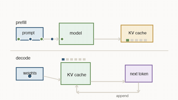
Decode is the loop you feel as streaming output. The model reads weights, reads the KV cache, computes the next token, appends new key/value state, and repeats. It cannot fully parallelize future tokens, because token 51 depends on token 50, which depends on token 49.

For each decode step, there are two basic timers competing:

• compute time: how long the matrix engines need to multiply through the active weights for the current batch
• memory time: how long memory needs to deliver the model weights and the KV cache vectors needed for attention

The token waits on whichever side is slower. That is why memory bandwidth, batch size, and cache placement matter so much.

Batch size means the serving system is running several users’ next-token steps together. The model weights are huge, but they are shared. If the system loads a block of weights and uses it for one user’s next token, that weight read was expensive for one result. If it uses the same loaded weights for many users in the same batch, the cost of that read is spread across many results.

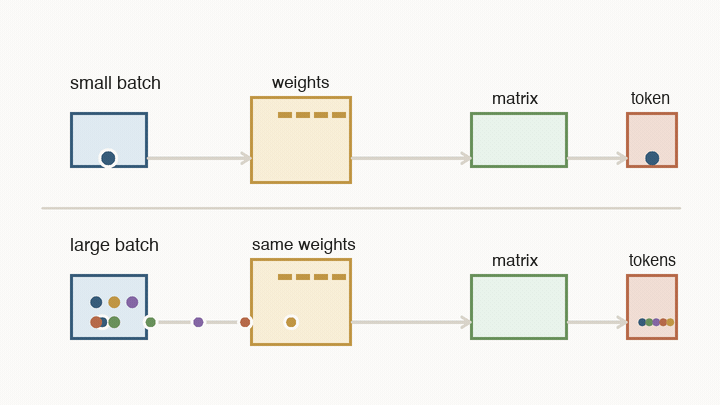
A small batch can start quickly, so it is good for low-latency streaming. But the hardware may spend a lot of time loading weights for very few tokens. A larger batch keeps the matrix engines busier and makes each weight read more useful, so cost per token falls. The price is that each user may wait longer for the batch to form and move through the decode loop.

Long context has the same physical shape. Extra tokens are not just text in a prompt. They become cached vectors. Every decode step may need to read back over more of that cache, so the bottleneck shifts toward memory capacity, memory bandwidth, and where the cache lives. A long-context model is not only “thinking about more text.” It is moving more remembered vectors through the serving system for every new token.

FPGA vs ASIC

The hardware trade-off also shows up in the choice between FPGAs and ASICs:

Choice	What it buys	What it costs
FPGA	Reprogrammability after manufacture, deterministic hardware behavior, fast prototyping	More routing overhead, lower density, lower efficiency
ASIC	Hard-wired efficiency, higher performance per watt, better density	High up-front cost, slower iteration, less flexibility

An FPGA uses lookup tables and programmable routing to imitate many possible circuits. An ASIC commits to one circuit. AI accelerators are mostly an ASIC bet: matrix multiplication, scratchpad memory, and structured communication are important enough to hard-wire.

The takeaway

Once you keep following the values, the chip starts to look less mysterious:

• A neural network repeats MAC operations.
• Lower precision can make each operation smaller.
• Data movement can cost more than the operation itself.
• Systolic arrays make reuse local and physical.
• Pipelines raise throughput by adding time boundaries, but they can add latency.
• Serving is shaped by the slower side of compute and memory.

So the next time an AI system feels fast, slow, cheap, or expensive, ask where the numbers are moving. Are weights being loaded for one request or many? Is the KV cache small enough and close enough to feed decode quickly? Is the model inside one fast scale-up domain, or are tokens waiting on pipeline stages across chips and racks?

AI hardware is not just about doing more math. It is about arranging memory, compute, and communication so the important numbers travel the shortest useful path.

Source: Reiner Pope’s blackboard lecture with Dwarkesh Patel, especially the YouTube version linked there.