Building a wildfire simulator with neural cellular automata

NCA Fireline is a small browser sim where fire spreads across a grid and cells try to draw their own fireline. The constraint is the point: no cell can see the whole map.

Press Step in the simulator. Fire starts as heat in a few squares. Nearby cells read that heat, mix it with fuel, moisture, wind, and hidden memory, and write new numbers back into the grid. After enough ticks, yellow risk appears ahead of the flame. When the neural cell rule is on, cyan fireline appears where the risk is high.

That is a neural cellular automaton. It is not one network looking at the whole map. It is one small network copied into every cell.

The linked simulator uses hand-initialized weights so the code stays readable. The training section later shows how those weights would be learned.

The Smallest Version

A cellular automaton is a grid plus a rule.

Each square has a state. At every tick, the rule looks at nearby squares and decides what this square should become next. Then every square updates at once.

Conway’s Game of Life is the usual example. A square is either alive or dead. The rule counts living neighbors. Too few neighbors, the cell dies. Too many, it dies. Exactly the right number, it lives or is born.

The code shape is almost boring:

for each cell:
  read nearby cells
  compute this cell's next state

replace old grid with next grid
repeat

There is no object called a glider in the rule. A glider appears because many small neighbor-counting updates keep handing the pattern forward.

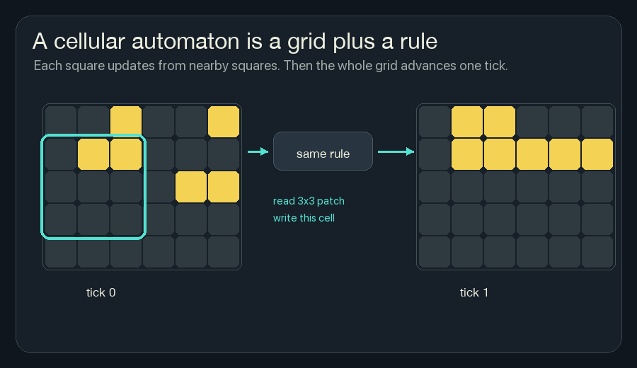
For the wildfire version, the state is not alive or dead. It is heat, fuel, moisture, risk, and fireline. But the loop is the same: read nearby cells, compute the next local state, repeat.

The Local Window

The simulator uses a 3x3 neighborhood. For one cell, that means:

• the cell itself,
• the three cells above,
• the two cells beside it,
• the three cells below.

That is all the cell can observe.

It cannot look across the grid and say, “The fire front is shaped like a hook.” It cannot know that the right side of the forest is still safe. It cannot plan a perfect firebreak. The cell gets a local patch and has to make a local update.

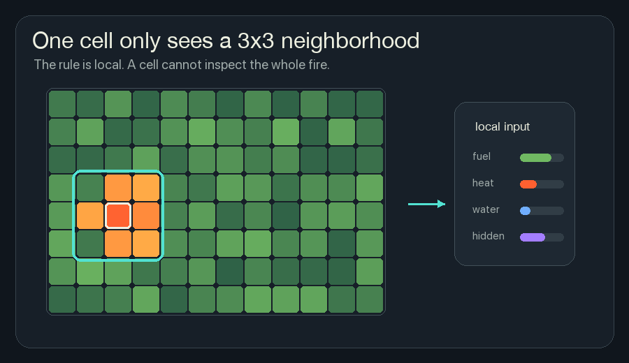
This restriction is why cellular automata are interesting. If a fireline forms ahead of the flame, it cannot be because one master cell saw the whole board. It has to come from local agreement: many cells read similar danger signals and write similar protection signals.

A Cell Carries Channels

A normal pixel has color. A simple cellular automaton might have one state: alive or dead, tree or fire, empty or full.

A neural cellular automaton cell carries a vector. That just means the cell stores several numbers at the same grid location.

In NCA Fireline, each cell has these channels:

Channel	Meaning
fuel	how much burnable material remains
heat	how strongly this cell is burning
moisture	how hard this cell is to ignite
burned	how much has already burned
retardant	water or fireline protection
ember	short heat memory
prediction	local estimate of near-future risk
hiddenA, hiddenB	scratchpad memory the renderer does not draw directly

The browser draws a composite view because I cannot show all those channels as one square without choosing colors. Green is fuel. Orange and red are heat. Yellow is risk. Cyan is retardant. Gray is burned ground.

But the rule is not reading “green” or “red.” It is reading numbers.

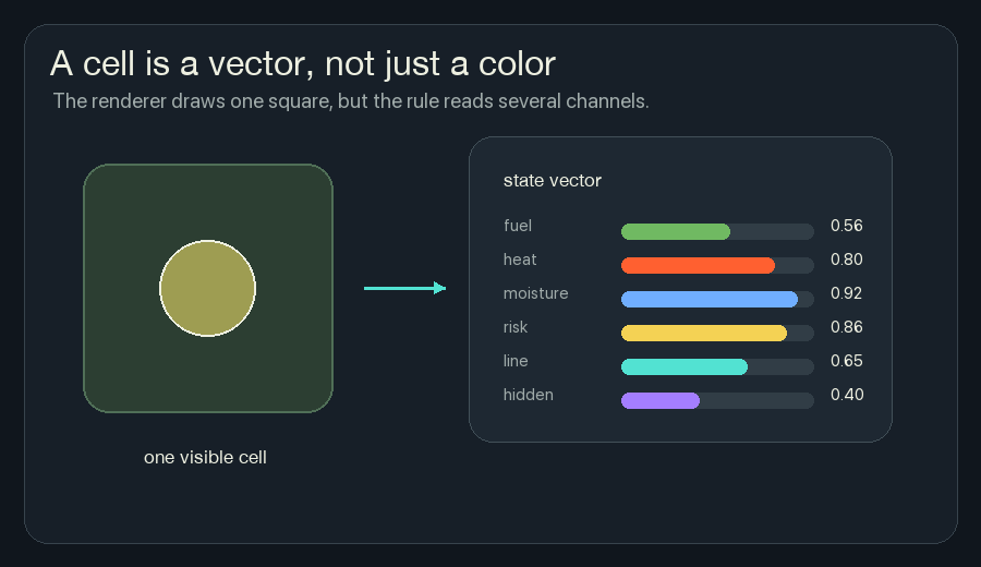
This one change makes the system much richer. A cell can be hot and wet. It can be burned but still remember recent heat. It can have fuel and high risk before it is actually on fire.

The next question is how those numbers change.

The Rule Is A Tiny Network

The word “neural” can sound huge, but an NCA rule can be very small.

For one cell, the rule receives the 3x3 neighborhood. In this simulator, that means nine cells, each with several channels. The rule mixes those local numbers and writes small changes back into this cell’s channels.

A neural network layer is just a set of weighted sums followed by a simple nonlinearity. The weights are knobs:

nearby heat  * positive weight  -> raises danger
wind heat    * positive weight  -> raises danger
fuel         * positive weight  -> raises danger
moisture     * negative weight  -> lowers danger
fireline     * negative weight  -> lowers danger
hidden trace * learned weight   -> depends on what training found useful

The nonlinearity keeps the result in a useful range. sigmoid squeezes a number between 0 and 1, which works well for a risk channel. tanh squeezes a number between -1 and 1, which works well for hidden signals that can push in either direction.

In a trained NCA, those weights are learned. In the browser version, the tiny network is present in the code, but the weights are chosen by hand so the mechanism can be read directly. The shape is still the same: local inputs in, mixed signals in the middle, channel changes out.

One output head can express a pattern like this:

risk goes up when:
  heat is nearby
  wind pushes heat toward this cell
  fuel remains
  hidden memory says this area has been active

risk goes down when:
  the cell is wet
  the cell has fireline
  the cell is already burned

That is not symbolic reasoning. The network is not thinking in sentences. It is turning local measurements into new numbers.

Repetition Moves Information

One update only moves information one neighborhood away.

If cell A is burning, the cells beside it can notice heat. On the next tick, those cells may heat up. Then their neighbors can notice. The fire front moves because the same local rule keeps running.

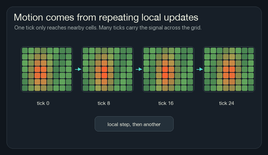
This is also why NCA can be hard to reason about from one line of code. The rule may be small, but it is applied many times. A tiny change in one channel can become visible after twenty or fifty updates.

Hidden Memory

Some channels are drawn. Some channels are not.

Hidden channels are scratchpad memory. They are numbers that live in the cell state and get copied forward, but the renderer does not need to show them as fuel or fire.

That matters because a purely instant rule can be jittery. It can only react to what is visible right now. A hidden channel lets the cell carry a trace: “heat was near me recently,” or “risk has been rising here,” or “this strip has started to become protected.”

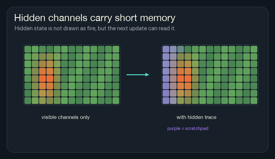
This is where the cell begins to feel less like a pixel and more like a tiny state machine. It still only sees locally, but it carries a small private history.

Prediction And Control

Prediction in this simulator is not a separate model. It is one channel in the cell vector.

Each tick, the rule writes a risk value into the prediction channel. A high risk value means: based on my local neighborhood, this cell is likely to become dangerous soon.

Once risk is a channel, control is just another local update:

if risk is high
and fuel remains
and this cell is not already protected:
  add some retardant

That writes into the retardant channel. When many cells do it, a cyan fireline appears ahead of the flame.

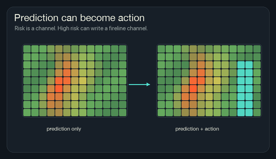
This is the game-like part of the project. You can paint heat, water, fuel, and line by hand. You can also turn on the neural cell rule and let local risk produce local protection.

Training Is The Important Part

The browser sim uses a tiny network, but the weights are hand-initialized. That makes the code easier to read, but it skips the most important question:

How would the network learn the rule instead of me writing it?

Training an NCA does not change the deployment story. A trained cell still only sees its local neighborhood. It still runs the same shared rule. It still writes channels back into the grid.

Training changes how we find the weights inside the rule.

Instead of me choosing constants like “nearby heat matters a lot” and “moisture should lower risk,” training starts with bad weights, runs the simulation, scores the result, and nudges the weights in the direction that would have produced a better result.

The trainable pieces are just the weight tables inside the local network:

3x3 local channels
  -> input weights
  -> hidden signals
  -> output weights
  -> next channels

At first those numbers are almost random. The rollout looks bad because the cell rule has not learned what heat, fuel, wind, memory, and fireline should mean together. Training is the loop that turns those anonymous numbers into a useful local habit.

The diagrams in this training section are conceptual. The playground linked above does not train in the browser; it uses fixed, hand-initialized weights so the local rule stays small enough to read.

That loop has five pieces.

1. Choose A Goal

Training needs a target. The target does not have to say what every cell should do at every tick. It can describe the final behavior we want.

For this wildfire simulator, a simple goal could be:

• keep heat from crossing a boundary,
• leave as much fuel alive as possible,
• use fireline only where it helps,
• avoid flickering or unstable channel values.

The target is not a secret map handed to each cell while the sim runs. It is only used by the training process to score the rollout.

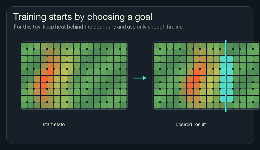
The trained rule can learn from global feedback during training. When it runs, each cell still gets only local observations.

2. Unroll Time

To train the rule, we run it for many ticks.

That is called unrolling. If the rule runs for 64 ticks, the training system keeps the chain:

state 0 -> state 1 -> state 2 -> ... -> state 64

Each arrow uses the same shared rule. The weights are reused at every tick and at every cell.

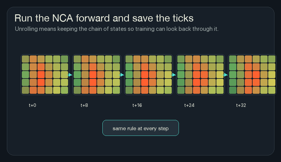
This is why NCA training can feel different from training a normal image classifier. The rule is not used once. It is used again and again, and the final behavior depends on the whole chain.

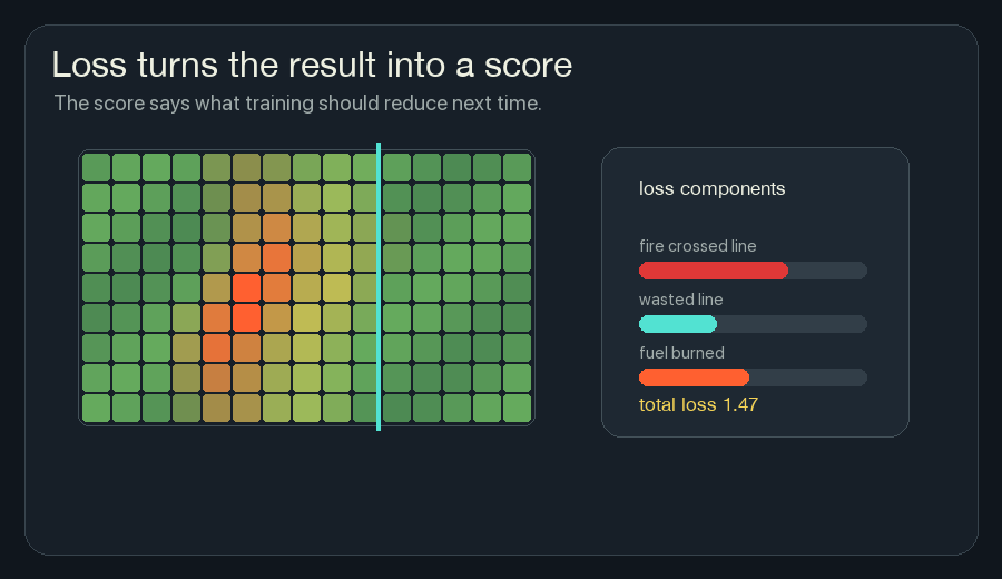
3. Calculate Loss

Loss is the number training tries to reduce.

If the final state is bad, the loss is high. If the final state is good, the loss is low.

For this wildfire version, a loss could be a weighted sum:

loss =
  heat that crossed the boundary
  + fuel that burned unnecessarily
  + fireline placed far away from risk
  + unstable flicker in hidden channels

The exact loss function is a design choice. If I punish fireline too strongly, the model may become timid and let fire through. If I punish burned fuel too strongly, it may paint too much line everywhere. Training does not remove the need to choose what “good” means.

This framing helped neural network training feel less abstract to me. The network does not start by knowing the rule. We define the score, then let many small updates search for weights that score better.

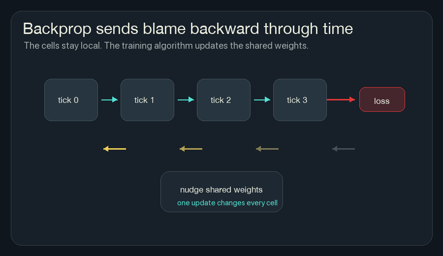
4. Backpropagate Through The Rollout

Backpropagation is bookkeeping for blame.

After the loss is computed at the end, backpropagation walks backward through the saved rollout and asks:

• which weights made the loss higher,
• which weights made the loss lower,
• how should each weight move a tiny amount?

Because the same rule is used at every cell and every tick, the gradients from many places add together. A gradient says how the loss changes when a weight moves. Gradient descent moves the weight the other way, toward lower loss. One weight might affect ignition near the left edge, prediction near the center, and fireline near the right edge. Training collects all of that pressure into one update for the shared rule.

This is the main reason training NCA is powerful. I do not have to decide by hand exactly how much wind heat should matter, or exactly how hidden memory should affect risk. If the loss is well-designed and the model is trainable, gradient descent can search those weights.

5. Update The Shared Rule

After backprop computes gradients, an optimizer changes the weights a little. An optimizer is the update recipe. It decides how large each nudge should be after the gradients point in a direction.

Then the whole process repeats:

start with random forest and wind
run the shared rule for many ticks
score the result
backpropagate through the ticks
update the weights
try again

The first rollouts are usually bad. Fire crosses the boundary. Prediction is late. Fireline appears in useless places. After many updates, the rule can start to discover useful local habits:

• risk should rise before heat arrives,
• fireline should appear near future danger,
• wet cells should resist ignition,
• hidden memory should smooth out local decisions,
• the rule should work across different wind and fuel patterns.

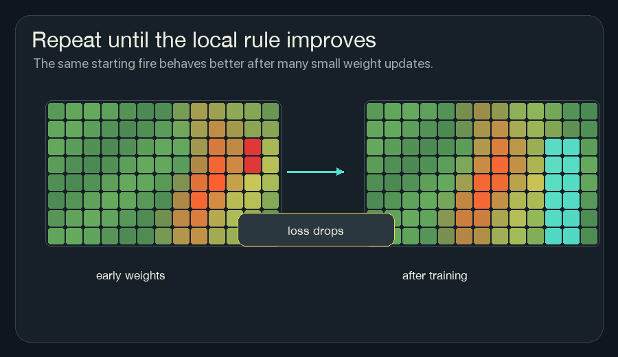
The trained weights are still just numbers in the tiny network. The cell still does not know the map. The global behavior comes from running the improved local rule many times.

Why Training Does Not Break Locality

This was the part that took me longest to understand.

During training, the loss can look at the whole grid. It can say, “fire crossed the boundary over there,” or “too much fuel burned overall.” That sounds global.

But the rule being trained is still local. The model does not learn a lookup table for one map. It learns weights for a function that each cell can run from its own neighborhood.

So there are two different views:

Phase	What can see the whole grid?	What the cell sees
Training	the loss function and backpropagation	still a local 3x3 neighborhood during each tick
Running the sim	nothing central has to act	the same local 3x3 neighborhood

That is the trick. Global feedback trains a local rule. Then the local rule creates behavior that looks coordinated.

The Playground Version

The playground keeps the mechanics visible.

The main field draws the composite state. The tabs let me inspect individual views: fuel, heat, risk, and line. The small channel previews show that the screen is not one image. It is several fields layered together.

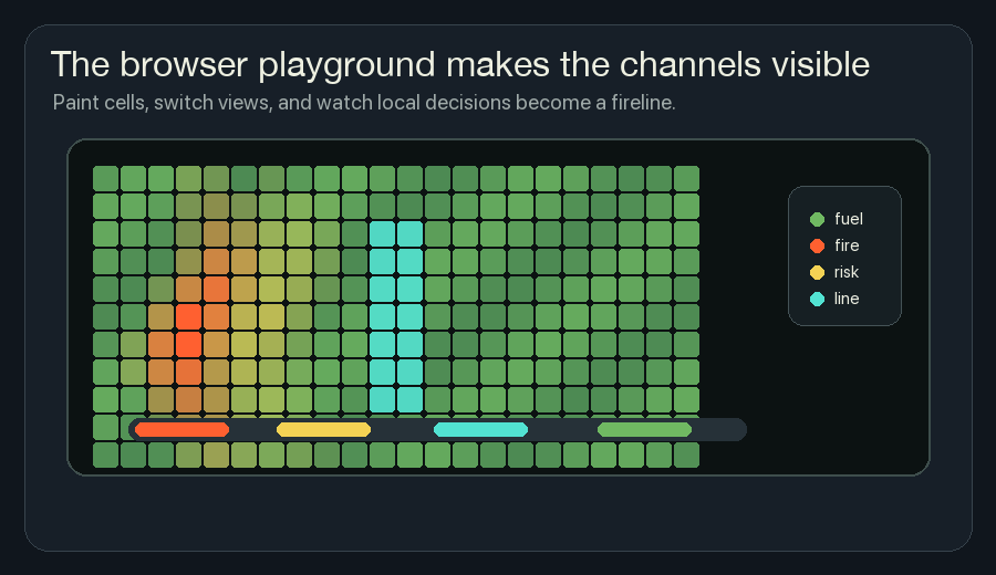
I like the playground most when it is paused.

Switch to risk and press Step a few times. Yellow appears before the orange front reaches it. Turn on the neural cell rule and step again. Cyan starts to appear in the same dangerous strip. Hover one cell there and the picture breaks back down into numbers: fuel, heat, risk, line, and memory.

That paused moment is the part I wanted. The picture turns back into one cell, one neighborhood, and a few numbers changing in order. The rest of the forest is still there, but I no longer have to explain it from above.