What training a tiny text-to-image model looks like

June 2, 2026

Text-to-image training is easier to understand when the word “image” disappears for a minute.

The training loop hands the model three things: a noisy grid of numbers, a number that says how noisy the grid is, and a text vector made from the caption. The model learns a direction for every part of that grid.

After training, generation starts from noise and walks those directions backward until the grid can be decoded into an image.

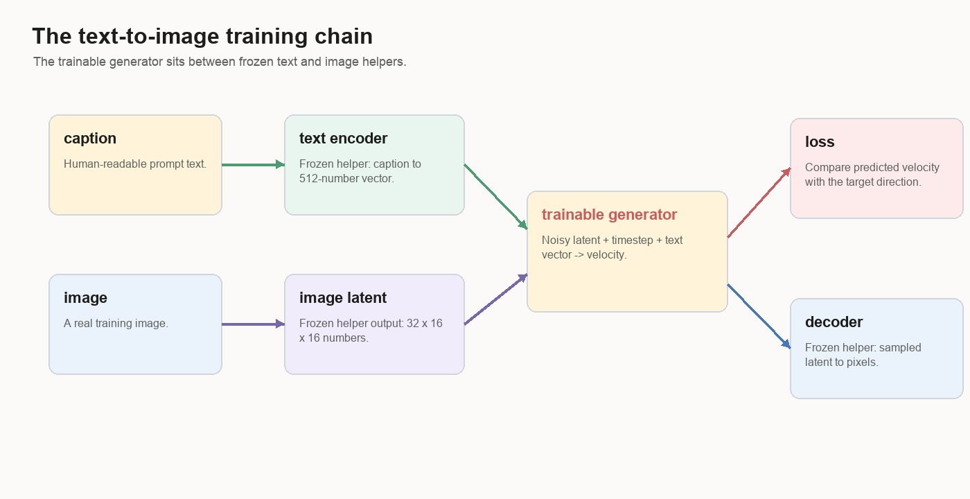
That is the system in monet-flow-tiny: a tiny latent flow text-to-image trainer, written to make the moving parts visible. The generator starts from random weights. The text encoder, image latents, and image decoder are frozen helpers, so the experiment can focus on one question:

Can a small generator learn to turn noise + text into an image latent?

The frozen helpers matter. A modern image model works as a chain of smaller jobs. Captions become vectors. Images become compressed latents. The generator learns a path through those latents. A decoder turns the final latent back into pixels.

A latent is the compact image grid the generator works on. It carries the layout and visual clues a decoder needs to make the final picture.

Diagram showing caption and image inputs, frozen text encoder, image latent, trainable generator, loss, and frozen decoder. — The trainable box is the generator. It learns in latent space. Frozen helpers turn captions into text vectors, turn images into latents, and turn sampled latents back into pixels.

This is a teaching-scale image model. Its value is the view into the training stack: what the data looks like, what the model sees, what flow matching trains, what sampling does, where Self-Flow-lite changes the task, and why image-like samples can still miss the prompt.

The Dataset Row

One training example has a human side and a tensor side.

The human side is an id and a caption. The tensor side is a text embedding and an image latent.

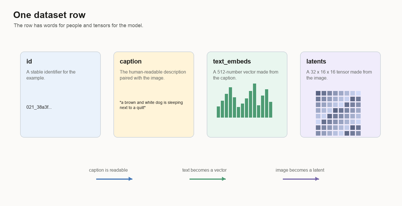
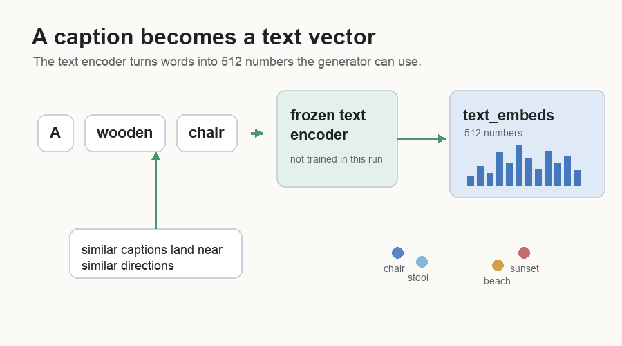
Diagram of one dataset row with id, caption, text_embeds, and latents fields. — The caption is readable prose. The text embedding and latent are numeric representations that let the model train on fixed-size tensors.

An embedding is just a useful numeric version of something. The text encoder is frozen: its weights stay fixed during this experiment. It reads the caption and returns a 512-number vector. That vector gives the caption numeric coordinates, and nearby directions in the vector tend to carry related meaning.

Diagram showing caption words flowing through a frozen text encoder into a 512-number text embedding, with nearby points in vector space representing related captions. — "A wooden chair" becomes a fixed-length list of numbers. The generator reads this vector during training.

In this project, the important shapes are:

text_embeds: 512 numbers
latents:     32 x 16 x 16 numbers

Shape means the layout of the numbers. A 512-number text embedding is one long list. A 32 x 16 x 16 latent is a stack of 32 small grids, each 16 by 16. Deep learning code calls both of these tensors. A tensor is an array of numbers with a shape attached to it.

During training, the generator reads the 512-number text vector. The JPEG has already been encoded into a 32-channel latent grid.

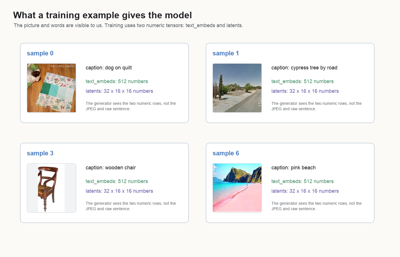
Four larger training example cards showing decoded target images, captions, text embedding shape, and latent shape. — These examples are readable to us as pictures and captions. The generator trains on the paired text vector and latent tensor.

This distinction matters because a text-to-image model has to bind text to visual structure through numbers. The phrase “wooden chair” becomes a vector. The chair image becomes a latent. The generator learns how those two numeric objects should interact.

Why Latents

Pixels are large.

A 512 by 512 RGB image has:

512 * 512 * 3 = 786432 values

The latent in this project has:

32 * 16 * 16 = 8192 values

That is about 96 times smaller.

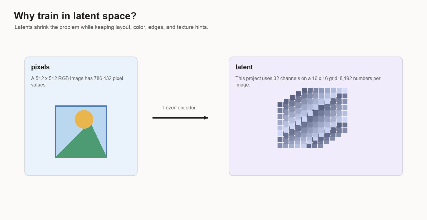
Diagram comparing a large pixel image with a smaller 32 channel 16 by 16 latent grid. — Latent space is a compressed image space. It carries layout, color, edge, and texture information in a smaller tensor.

Latent means hidden representation. Here it is hidden only because it lives between two visible things:

image pixels -> frozen encoder -> latent -> frozen decoder -> image pixels

The latent is the middle form. It keeps enough information for the decoder to rebuild an image, but it is much smaller than the original pixel grid. You can think of it as a compact working space for images.

Training in latent space makes the project small enough to study. The frozen decoder handles low-level pixel decoding, like how nearby red, green, and blue pixel values make an edge or a texture. The generator’s job is narrower:

noise + time + text vector -> image-like latent

That narrower job is still hard. The latent grid has to contain object layout, scene composition, color, lighting, and texture hints. It also has to change when the caption changes.

The Generator

The generator is the only part being trained. Plainly, it does four jobs:

split the latent into patches
let patches compare with other patches
mix in the caption and noise level
predict a direction for every latent value

The architecture is a small DiT-style transformer over latent tokens. DiT means diffusion transformer: instead of using a transformer only for text, use transformer blocks on image-like tokens while a denoising or flow model is being trained.

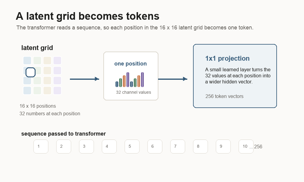
A transformer reads a sequence. The latent starts as a grid. The first job is to turn the grid into a sequence the transformer can read.

The latent grid is 16 x 16. That gives 256 spatial positions. At each position, there are 32 channel values. The code treats each spatial position as one token. So one image latent becomes a sequence of 256 tokens.

A 1x1 projection is the small learned layer that prepares each token for the transformer. It looks at the 32 values at one grid position and turns them into a wider hidden vector. The model also adds a position embedding, which is a learned address for row and column. The address tells the transformer where each token sits in the image grid.

Diagram showing a 16 by 16 latent grid becoming 256 transformer tokens through a 1 by 1 projection. — One latent position becomes one token. The projection turns that position's 32 channel values into the hidden vector size used by the transformer.

The text vector and timestep enter as conditioning. Conditioning means control information. The latent tokens carry the current image state. The text vector says what the image should become. The timestep says how noisy the current latent is. Inside each DiT block, the conditioning signal shifts and scales the token features so the same latent can be updated differently for different prompts and noise levels.

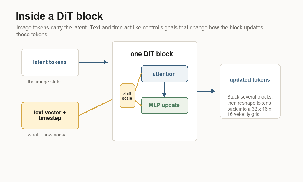
Diagram showing latent tokens entering one DiT block while text and timestep conditioning shift and scale the attention and MLP update. — The image information flows through the token stream. Text and time act like control signals that change how each DiT block updates that stream.

Attention is the part of the block that lets tokens compare with other tokens. A noisy patch near the middle of a chair can borrow clues from nearby patches that look like a back, seat, floor, or wall.

Animated diagram showing one latent token attending to nearby latent tokens before predicting a velocity direction. — Attention lets a patch use context. The patch still gets its own velocity prediction, but that prediction can depend on other patches in the latent.

The MLP layers inside the block update each token after attention mixes context. An MLP is a small stack of learned linear layers and nonlinearities. It is the part that reshapes the features after the token has gathered information.

That gives the model a way to answer local questions:

This patch is noisy.
The timestep says it is very noisy.
The caption vector points toward a chair scene.
The surrounding patches suggest a chair back.
Which direction should this patch move?

The velocity head turns the final tokens back into a 32 x 16 x 16 tensor. It predicts a direction for every latent value. When Self-Flow-lite is enabled, an auxiliary head also tries to reconstruct clean latents from an internal layer. More on that later.

Flow Matching

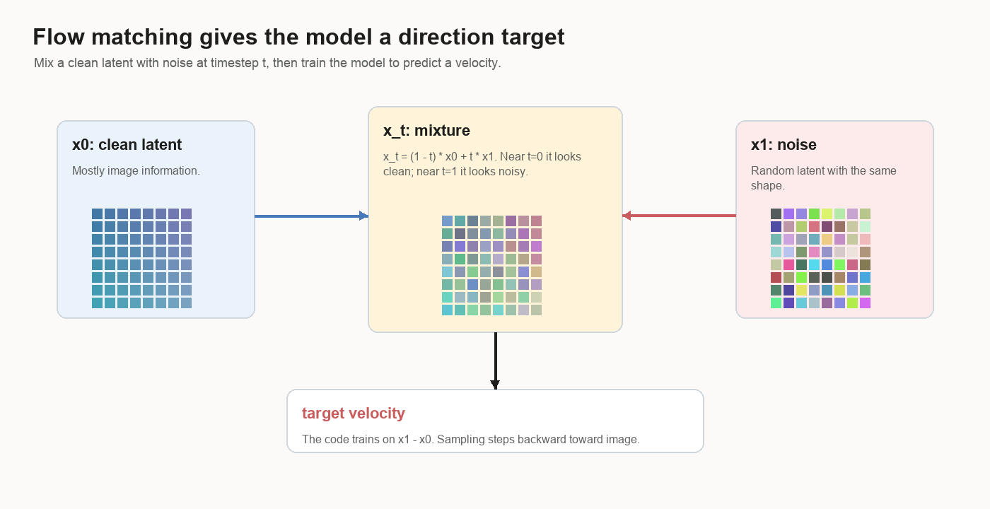
Flow matching gives the model a supervised target at every training step.

The name comes from the picture: imagine every possible noisy latent has an arrow attached to it. The arrow says which way that point should flow. Training matches the model’s predicted arrow to the arrow computed from clean latent and noise.

Start with a clean image latent:

x0 = clean latent

Pick random noise with the same shape:

x1 = noise

Pick a timestep between 0 and 1:

t = random number

Mix the two:

x_t = (1 - t) * x0 + t * x1

Near t = 0, the mixture is mostly image. Near t = 1, it is mostly noise.

The code trains the model to predict:

target_velocity = x1 - x0

Velocity means direction plus size. If the clean latent is here and the noise is over there, the target velocity is the arrow from clean to noise. The model sees the mixed latent x_t, the timestep t, and the caption vector. It has to guess that arrow.

That is the clean-to-noise direction. Sampling starts at noise and steps backward against that learned field, so the sampled latent moves from noise toward image.

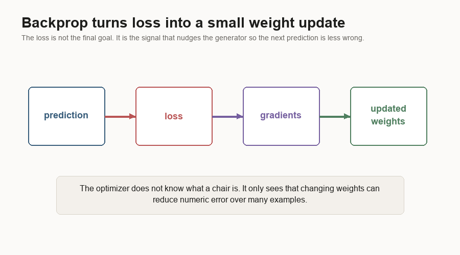
Diagram showing x0 clean latent, x1 noise, x_t mixture, and target velocity x1 minus x0. — Training teaches the direction from clean latent to noise. Generation uses the same learned field in reverse.

The loss is mean squared error between the predicted velocity and the target velocity.

Loss is the training score the optimizer tries to reduce. It answers a narrower question than human image quality:

How far is the model's predicted arrow from the arrow we can compute?

Mean squared error means:

prediction - target
square the difference
average the squared differences

That sounds plain, but it creates a dense learning signal. The model gets feedback for every latent value, rather than one label for the whole image.

Animated diagram showing target velocity arrows and model-predicted velocity arrows becoming closer as mean squared error loss shrinks. — The target arrows are computed from clean latent and noise. The predicted arrows come from the generator. Loss is the average mismatch.

Backpropagation is the bookkeeping that asks which weights contributed to the error. The result is a gradient: a direction for changing each weight so the loss should go down a little. The optimizer then nudges those weights by a small amount. The optimizer sees numeric error. Chair-like behavior emerges only after many examples push those numbers in useful directions.

Diagram showing prediction feeding loss, loss producing gradients, and gradients updating generator weights. — Loss becomes gradients. Gradients become small weight updates. Repeat this enough times and the generator's velocity field starts to match the data.

Sampling

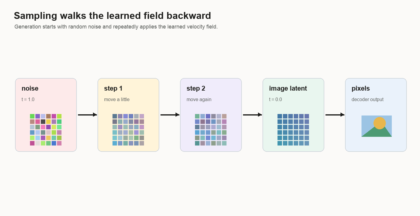
After training, sampling begins with random noise:

latents = random noise

Sampling is a walk. The model predicts a small velocity step, the sampler moves the latent, then the next step asks the model again.

Animated diagram showing sampling as repeated steps from t equals 1 noise toward a t equals 0 image latent. — The caption vector stays the same across the walk. The latent and timestep change at every step.

For each step, the sampler asks:

Given this latent, this timestep, and this text vector,
what velocity does the model predict?

Then it takes a small step backward:

latents = latents + dt * velocity

where dt is negative because sampling walks from t = 1 to t = 0.

Diagram showing sampling from noise through intermediate steps to an image latent and decoded pixels. — Sampling is iterative. The model repeatedly nudges the latent, then the decoder turns the final latent into pixels.

The sampler also has a prompt-strength knob. It asks: what changed when the text was present, and how hard should sampling push in that direction?

The usual name for this family of tricks is classifier-free guidance. The name comes from an older steering method that used a separate classifier to push the image toward a class label. Classifier-free guidance removes that extra classifier. The image model itself learns two modes: a prompt mode and a blank text mode.

Full classifier-free guidance trains both modes. During training, some captions are replaced with blank text, so the blank-text prediction becomes a reliable reference. The configs here keep text dropout at 0.0, so the blank-text branch has little training signal. That makes the guidance knob useful as a prompt-sensitivity probe for this project, while full guidance would need training examples with blank text.

At sampling time, the model can still be run twice:

unconditioned = model(latent, t, zero_text)
conditioned   = model(latent, t, prompt_text)

The sampler then pushes away from the unconditioned prediction:

guided = unconditioned + scale * (conditioned - unconditioned)

The intuition is simple: ask the model what it would do with blank text, ask what it would do with the prompt, then exaggerate the difference made by the prompt.

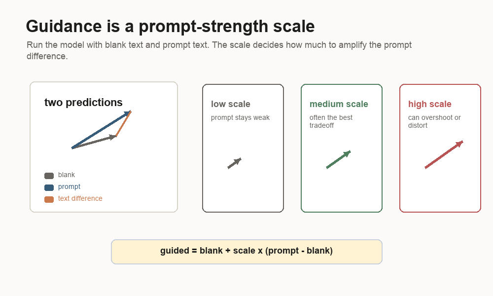
Diagram showing blank and prompt velocity predictions, then low, medium, and high guidance scale effects. — Low scale lets the image prior dominate. Medium scale often gives the best prompt/image tradeoff. High scale can overshoot and distort the latent.

Low guidance means a small scale. The image tends to stay stable, and the prompt can stay weak. High guidance means a large scale. The text difference gets amplified, which can make samples more dramatic and can also push the latent into distorted directions. In these runs, stronger guidance often made samples more dramatic while still missing the requested subject.

Self-Flow-lite

Self-Flow-lite uses the same generator with a harder training recipe.

The baseline uses one timestep for the whole latent.

all patches use t = 0.63

Self-Flow-lite makes the training example uneven:

patch 1 uses t = 0.10
patch 2 uses t = 0.75
patch 3 uses t = 0.40
...

It also masks or heavily corrupts some patches by setting them to a high noise timestep. The model still has to predict the velocity field.

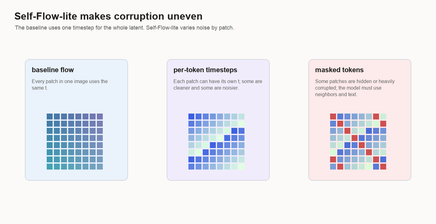
Diagram comparing baseline flow, per-token timesteps, and masked tokens. — Normal flow gives the whole latent one noise level. Self-Flow-lite gives different patches different noise levels, then corrupts a subset harder.

The point is to stop the example from being uniformly easy or uniformly hard. In the baseline, every patch in the latent has the same noise level. With Self-Flow-lite, one patch may be nearly clean, another may be mostly noise, and some masked patches may be pushed all the way to t = 1.0.

That forces the model to use context. If one patch is heavily corrupted, the nearby patches and the caption become more important.

The auxiliary loss adds another pressure. An auxiliary head is a small side prediction head attached to an internal layer of the generator. It tries to reconstruct the clean latent. When masked-only mode is enabled, the reconstruction loss is computed only on the masked tokens. That auxiliary loss is multiplied by a weight and added to the velocity loss.

Animated diagram showing clean latent patches, corrupted masked patches, and an auxiliary reconstruction moving masked patches back toward the clean latent. — The auxiliary head is a training-time teacher signal. It asks the model's internal representation to recover clean masked patches, while the main head still predicts velocity.

So Self-Flow-lite changes the task in three concrete ways:

per-token timesteps
masked or heavily corrupted patches
auxiliary clean-latent reconstruction

Animated diagram showing latent patches getting per-token timesteps, masks, and flow plus reconstruction losses. — The hope is concrete: uneven corruption forces the model to use nearby patches, text, and learned structure instead of one global cleanup shortcut.

That harder task can help the numeric objective because the model gets more varied denoising situations and an extra reconstruction signal. Prompt following remains a separate skill. A model can improve at latent cleanup while still struggling to bind the word “chair” to a chair-shaped region.

What Training Looks Like

The first useful question is:

Does the loop work?

A synthetic smoke test checks shapes, model forward pass, loss, optimizer, checkpoints, and validation. It proves the code path runs. It says nothing about image quality.

The next question is:

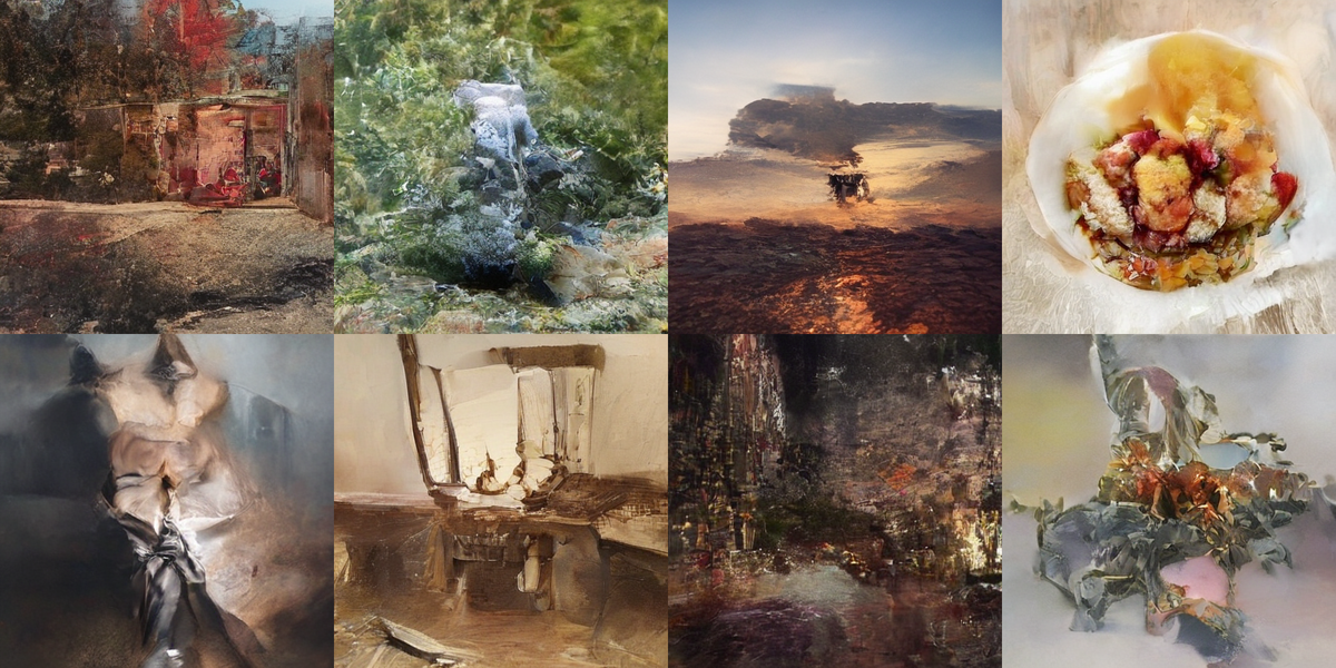
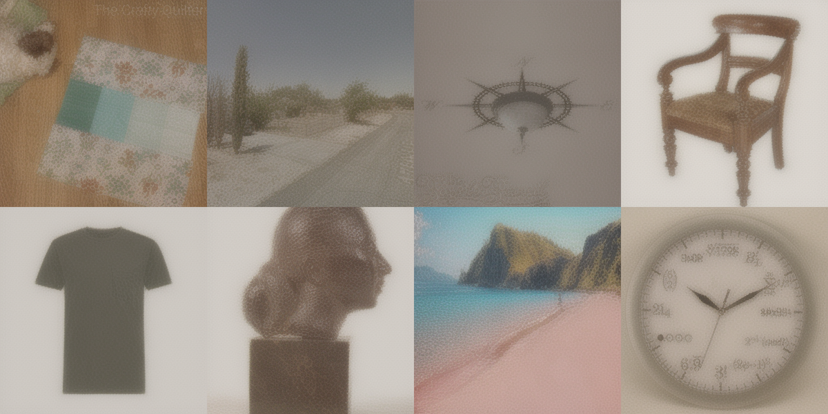
Can the code load real MONET latents and text vectors?

Early samples from tiny real runs look like texture. That is normal. A working training loop can still be far from a working image model.

Early tiny baseline sample grid with mostly texture-like generated outputs. — Early generated grids can be useful even when they are ugly. This kind of texture tells me the sampler and decoder are producing images while meaningful objects are still forming.

Validation loss is the velocity loss measured on examples held out from training. It helps catch whether the model is improving beyond the exact batches it just saw. It is still a velocity-matching number, while prompt-following needs visual inspection.

On a small filtered subset, the baseline and Self-Flow-lite both still produced weak early samples. Self-Flow-lite improved that held-out velocity-loss number in the small comparison, while the images still failed to bind prompts to objects.

Small filtered baseline sample grid at step 1000. — Baseline, small filtered subset, early checkpoint. The grid is image-texture rather than object structure.

Small filtered Self-Flow-lite sample grid at step 1000. — Matched Self-Flow-lite run, early checkpoint. A lower loss still left prompt coherence weak.

That is the first important lesson from the experiment:

lower velocity loss and prompt-coherent images are separate milestones.

Loss tells whether the model is learning the numeric target. Samples tell whether the learned field decodes into useful images.

Fixed-prompt samples answer a different question. You keep the prompts, starting noise, sampler settings, and checkpoint cadence the same. Then you look at whether the same requests become clearer and more prompt-aligned over time.

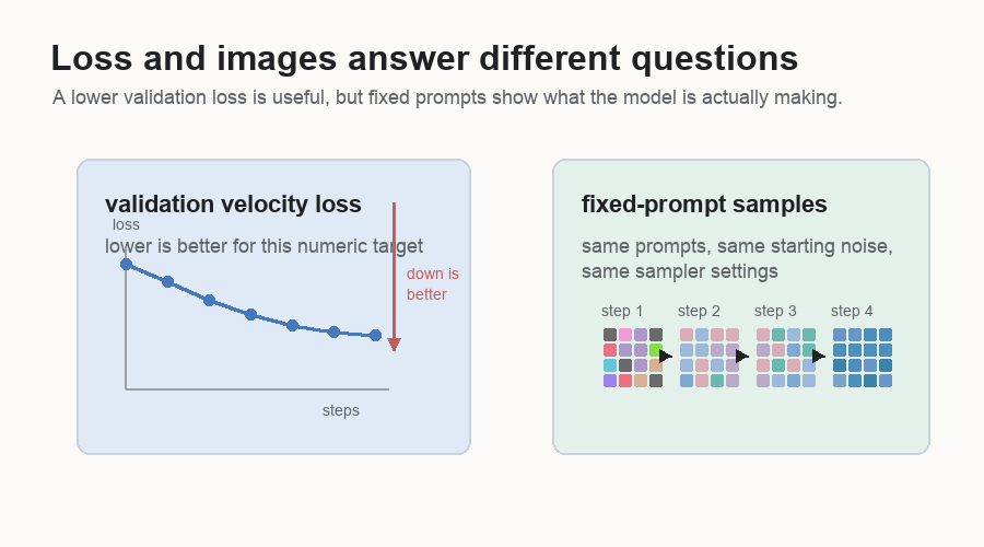
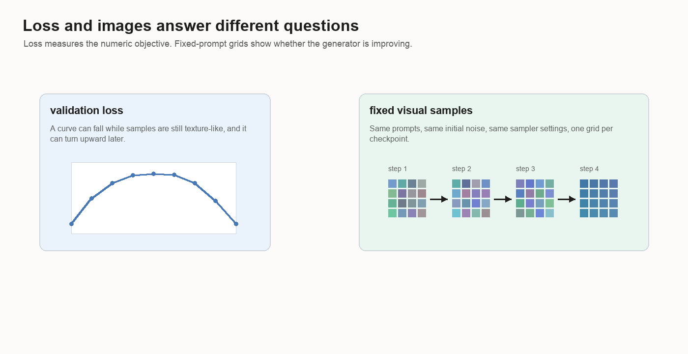
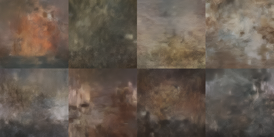
Diagram comparing a validation loss curve with a fixed-prompt sample grid, showing that loss and samples answer different questions. — Validation loss checks the numeric target. Fixed-prompt grids check whether the learned directions turn into the right visible content.

Diagram comparing validation loss with fixed visual sample grids over checkpoints. — The training runs track both loss and fixed-prompt samples. The visual grid uses the same prompts, same starting noise, and same sampler settings at each checkpoint.

Image-Like Comes Before Prompt-Coherent

The broader run did learn an image prior.

An image prior means the model has learned something about what images tend to look like: color fields, lighting, depth, object-like regions, interiors, landscapes, and material texture.

Animated progress grid from a broader text-to-image training run, showing samples becoming more image-like over checkpoints. — The broader run moves from texture toward image-like scenes. The samples are moving beyond random texture, while the prompts are still weakly bound to the output.

Prompt coherence is stricter.

An image is prompt-coherent when the requested subject or scene appears, and when changing the prompt changes the content in the expected way. A model can learn lighting, texture, and composition before it learns that “chair” should create a chair-shaped object.

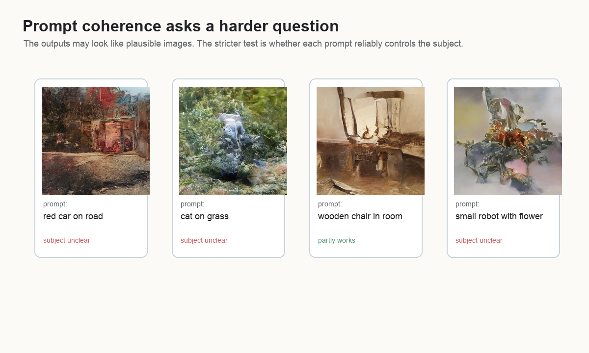
Broad training run sample grid with image-like but weakly prompt-coherent results. — A later broad-run grid has landscapes, object-like blobs, interiors, and lighting. It is image-like, with unreliable prompt coherence.

Diagram showing generated image-like samples next to prompts such as red car on road, cat on grass, wooden chair in room, and small robot with flower, with several subjects marked unclear. — The failure is weak control. The model can make plausible image texture while missing the requested subject.

That distinction became the clearest result of the project.

image-like:        this looks like something from the image distribution
prompt-coherent:   this matches the caption in the intended way

The broad model reached the first stage and stayed short of the second.

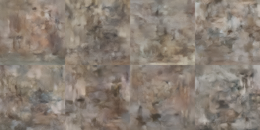
Why The Overfit Run Matters

When a broad model is weak, too many explanations are possible:

the sampler is wrong
the decoder scale is wrong
the objective is wrong
the architecture is too small
the dataset is too broad
the text conditioning is too weak

An overfit run removes some of that ambiguity.

The question is simple:

Can the model memorize a small visual world?

Overfitting usually means a model has memorized the training data too closely and generalizes poorly. That is bad when the goal is a useful model. Here it is a diagnostic tool. If 512-example memorization fails, the broad dataset is probably one explanation among several. Something more basic may be wrong.

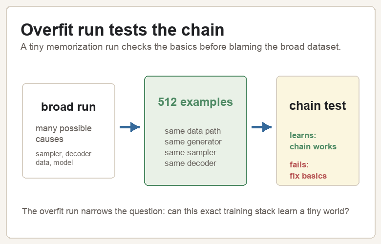
Diagram showing a broad run narrowed to a 512-example memorization run to test whether the training chain works. — The overfit run removes variety on purpose. It asks whether the chain can learn a tiny world before asking it to generalize to a broad one.

A 512-example run reproduced that narrow world clearly. The point was to test whether the training stack can learn at all.

Reference grid from the 512 example overfit subset, showing target images such as a dog near a quilt, a street, a chair, a shirt, a bust, a beach, and a clock. — The tiny overfit world: a dog next to a quilt, a street, a ceiling graphic, a chair, a shirt, a bust, a beach, and a clock.

Animated progress grid from a 512 example overfit run, showing generated samples becoming clearer over training steps. — In the overfit run, the same tiny world gets clearer over checkpoints. This is the strongest evidence that the data path, model, sampler, and decoder are part of a working training chain.

Final generated grid from the 512 example overfit run, showing coherent images from the tiny subset. — Final 512-example overfit grid. The model can produce coherent images when the world is small enough.

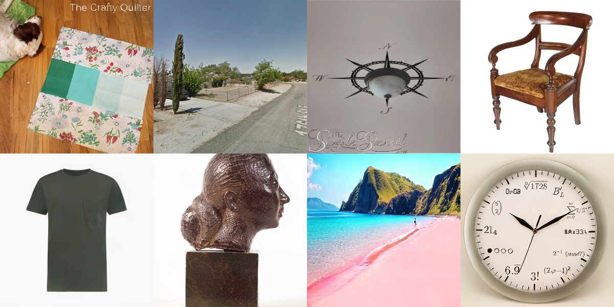
Once the overfit run works, the broad failure becomes more specific. The decoder can show valid latents. The sampler can walk the learned field. The generator has enough capacity to memorize a small set. The remaining weakness is broad generalization and prompt binding.

The Next Dataset

The next run should do more than train the same broad dataset for more steps. It should make prompt binding easier first.

A cleaner staged dataset would look like this:

category: chair
prompt:   a wooden chair

category: dog
prompt:   a dog on a blanket

category: beach
prompt:   a beach with blue water

category: clock
prompt:   a round wall clock

Short prompts and repeated categories would give the model a simpler first job: bind nouns to shapes. After that works, longer captions can come back.

That is the practical next step:

first learn nouns
then learn attributes
then learn full scenes

Self-Flow-lite can still be useful in that setup. The right comparison is a matched baseline and Self-Flow-lite run on the same curated subset, with the same fixed-prompt monitoring grid and the same sampler settings.

The Chain

Text-to-image training is a chain.

dataset row
  -> caption vector + image latent
  -> mix clean latent with noise
  -> generator predicts velocity
  -> loss updates generator
  -> sampling starts from noise
  -> generated latent
  -> decoder makes image

Every link matters: data, captions, latents, conditioning, objective, architecture, sampler, decoder, and monitoring.

The tiny overfit run shows the chain can work. The broad run shows the next hard part: getting the model to follow the prompt instead of only making something image-like.

That is the useful boundary. Once the system can learn a tiny world, the question moves from “does training work?” to “how do I make text control strong enough to survive a broader world?”

The code for the project is here: silentvoice/monet-flow-tiny.